ENGINEERING HYDROLOGY: CHAPTER 061 - STATISTICAL DISTRIBUTIONS

1. CONCEPTS OF STATISTICS

1.01
Statistical hydrology uses random variables and probability distributions.

1.02
A random variable follows a certain probability distribution.

1.03
A probability distribution is a function that expresses in mathematical terms the relative chance of occurrence of each of all possible outcomes of the random variable.

1.04
P(X = x_i) is the probability P that the random variable X takes on the outcome x_i.

1.05
A shorter notation is P(x_i).

1.06
An example of random variable and probability distribution is shown here.

1.07

1.08
This is a discrete probability distribution because the possible outcomes have been arranged into groups or classes.

1.09
The random variable is discharge Q.

1.10
The possible outcomes are seven classes, from 1-100 to 600-700 m3/s.

1.11
In this figure, the probability that Q is in the class 100-200 is 0.25, or 25%.

1.12
The sum of probabilities of all possible outcomes is 1, or 100%.

1.13
A corresponding cumulative discrete distribution is shown here.

2.14

1.15
In this figure, the probability that Q is in a class less than or equal to the 100-200 class is 0.40, or 40%.

1.16
The maximum value of probability of the cumulative distribution is 1, or 100%.

2. PROPERTIES OF DISTRIBUTIONS

2.01
The properties of statistical distributions are described by the following measures: (1) central tendency, (2) variability, and (3) skewness.

2.02
Statistical distributions are described in terms of moments.

2.03
The first moment describes central tendency, the second moment describes variability, and the third moment describes skewness.

2.04
The first moment about the origin is the arithmetic mean, mean, or average.

2.05
It expresses the distance from the origin to the centroid of the distribution, as shown here.

2.06
The B distribution has a higher mean that the A distribution.

2.07
The formula for the mean is:

2.08

- 1 _n

x =

∑

x_i

n ⁱ⁼¹

2.09
in which x_ is the mean, x_i is the random variable, and n is the number of values.

2.10
The geometric mean is the n^th root of the product of n terms:

2.11

-
x_g = (x₁ x₂ x₃ ... x_n)^1/n

2.12
The logarithm of the geometric mean is the mean of the logarithms of the individual values.

2.13
The geometric is to the lognormal probability distribution what the arithmetic mean is to the normal probability distribution.

2.14
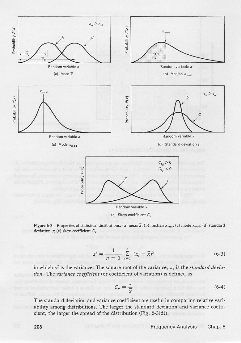
The median is the value of the variable that divides the probability distribution into two equal portions, as shown here.

2.15
For certain skewed distributions, that is, those with third moment other than zero, the median is a better indication of central tendency than the mean.

2.16
Another measure of central tendency is the mode, defined as the value of the variable that occurs most frequently, as shown here.

2.17
Statistical moments can be defined about axes other than the mean.

2.18
The second moment about the mean is the variance, defined as follows:

2.19

1 _n

s² =

∑

(x_i - x)²

n-1 ⁱ⁼¹

2.20
in which s² is the variance.

2.21
The square root of the variance, that is, s, is the standard deviation.

2.22
The coefficient of variation, or variance coefficient, is defined as follows:

2.23

s
C_v =
x -

2.24
The standard deviation and coeficient of variation are useful in comparing the relative variability among distributions.

2.25
The larger the standard deviation and coefficient of variation, the larger the spread of the distribution.

2.26
In this figure, the standard deviation of distribution C is larger than that of D.

2.27
The third moment about the mean is the skewness, defined as follows:

2.28

1 _n

a =

∑

(x_i - x)³

(n-1)(n-2) ⁱ⁼¹

2.29
in which a is the skewness.

2.30
The skew coefficient is defined as follows:

2.31

a
C_s =
s³

2.32
For symmetrical distributions, the skewness is zero and the skew coefficient C_s is zero.

2.33
For right skewness, with distribution with long tail to the right, C_s is greater than 0.

2.34
For right skewness, with distribution with long tail to the left, C_s is less than 0.

2.35

3. NORMAL DISTRIBUTION

3.01
A continuous probability function is referred to as a probability density function or PDF.

3.02
A PDF is an equation relating probability, random variable, and parameters of the distribution.

3.03
Selected PDFs useful in engineering hydrology are the normal, the Pearson Type III, and the Extreme Value.

3.04
The normal distribution is a symmetrical, bell-shaped PDF also known as the Gaussian distribution, or the natural law of errors.

3.05
It has two parameters: (1) the mean μ, and (2) the standard deviation σ, of the population.

3.06
In practical applications, the mean x_ and the standard deviation s derived from sample data are substituted for μ and σ.

3.07
The PDF of the normal distribution is:

3.08

f(x) =

e^{-(x - μ)²/(2&sigma²)}

σ (2π)^1/2

3.09
in which X is the random variable and f(x) is the continuous probability.

3.10
By means of the transformation:

3.11

x - μ
z =
σ

3.12
the normal distribution converts into the following one-parameter distribution:

3.13

f(x) =

e^-z²/2

(2π)^1/2

3.14
in which z is the standard unit, which is normally distributed with zero mean and unit standard deviation.

3.15
Solving for x:

3.16

x = μ + z x

3.17
in which the standard unit z is the frequency factor of the normal distribution.

3.18
In general, the frequency factor of a statistical distribution is referred to as K.

3.19
Thus, for the normal distribution: K = z.

3.20
Integration of the one-parameter normal probability density function leads to the cumulative density function, or CDF, of the normal distribution:

3.21

1 z

F(z) =

∫ e^-u²/2 du

(2π)^1/2 -∞

3.22
in which F(z) denotes cumulative probability and u is a dummy variable of integration.

3.23
The distribution is symmetrical with respect to the origin.

3.24
Therefore, only half of the distribution needs to be evaluated.

3.25
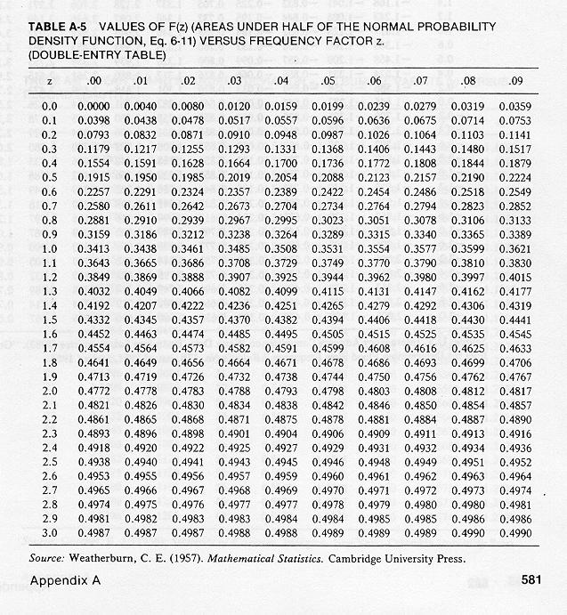
Values of F(z) vs z are shown in this table.

3.26

3.27
In this table, note that for z = 1, f(z) = 0.3413, that is, 34.13% of the normal distribution probability lies between the mean and one standard deviation away from the mean.

3.28
Likewise, for z = 2, f(z) = 0.4772, that is, 47.72% of the normal distribution probability lies between the mean and two standard deviations away from the mean.

4. PEARSON TYPE III DISTRIBUTION

4.01
The Pearson Type III distribution has been widely used in flood frequency analysis.

4.02
It is a three-parameter skewed distribution with the following PDF:

4.03

(x - x_o)^{γ -1} e^-(x-x_o)/β
f(x) =
β^λ Γ(γ)

4.04
and parameters β, γ, and x_o.

4.05
The term Γ(γ) is an important definite integral referred to as the gamma function.

4.06
It is defined as follows:

4.07

∞

Γ(γ) =

∫ x^γ-1 e^-x dx

4.08
The mean of the Pearson Type III distribution is:

4.09

μ = x_o + β γ

4.10
The variance is:

4.11

s² = β² γ

4.12
The skewness is:

4.13

a = 2/(γ)^1/2

5. EXTREME VALUE DISTRIBUTIONS

5.01
Extreme value theory has been used in frequency analysis since the 1920s.

5.02
Extreme value theory implies that if a random variable Q is the maximum of a sample of size n from some population of x values, then, provided n is sufficiently large, the distribution of Q is one of three asymptotic types, I, II or III, depending on the distribution of x.

5.03
The extreme value distributions can be combined into one and expressed as a general extreme value, or GEV distribution.

5.04
The cumulative density function of the GEV distribution is:

5.05

F(x) = e^{-[1 - k(x-u)/α]^1/k}

5.06
in which k, u, and α are parameters.

5.07
The parameter k defines the type of distribution, the parameter u defines the location, and the parameter α relates to scale.

5.08
For k = 0, the GEV distribution reduces to the Extreme Value Type I, or Gumbel, distribution.

5.09
For k < 0, the GEV distribution is the Extreme Value Type II, or Frechet, distribution.

5.10
For k > 0, the GEV distribution is the Extreme Value Type III, or Weibull, distribution.

5.11
Gumbel has fitted the extreme value Type I distribution to long records of river flows for many countries.

5.12
The cumulative density function of the Gumbel distribution is the following double exponential function:

5.13

F(x) = e^{-e^-y}

5.14
in which y is the Gumbel variate, defined as follows:

5.15

x - u
y =
α

5.16
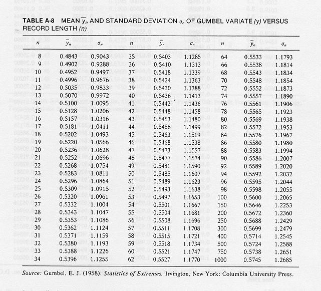
The mean and standard deviations of the Gumbel variate are functions of the record length n.

5.17
This table shows mean and standard deviations of the Gumbel reduced variate y, as a function of record length n.

5.18
When the record length approaches infinity, the mean of the Gumbel variate approaches asymtotically the Euler constant, that is, 0.5772. and the standard deviation approaches the value of π over square root of 6, that is, 1.2825.

5.19
The skew coefficient of the Gumbel distribution is 1.14.

5.20

Narrator: Victor M. Ponce

Music: Fernando Oñate

Editor: Flor Pérez

Visualab Productions