1. SELECTION OF DATA SERIES

1.01
The complete record of streamflows at a given gaging station is called the complete duration series.

1.02
To perform a flood frequency analysis, it is necessary to select a flood series, that is, a sample of flood events extracted from the complete duration series.

1.03
There are two types of flood series: (1) partial duration series, and (2) extreme value series.

1.04
The partial duration series consists of floods whose magnitude is greater that a certain base value.

1.05
When the base value is such that the number of events in the series is equal to the number of years of record, the series is called an annual exceedence series.

1.06
The partial duration series is also referred to as peaks-over-a-threshold, or POT series.

1.07
In the extreme value series, every year of record contributes one value to the extreme series, either the maximum, as in the case of flood frequency analysis, or the minimum value, as in the case of low-flow frequency analysis.

1.08
The former is the annual maxima series.

1.09
The latter is the annual minima series.

1.10
The difference between annual exceedence and annual maxima series is likely to be more marked for short records, in which the second largest annual events may strongly influence the character of the annual exceedence series.

1.11
In practice, the annual exceedence series is used for frequency analyses involving short return periods, ranging from 2 to 10 years.

1.12
For longer return periods, the difference between annual exceedence and annual maxima series is small.

1.13
The annual maxima series is used for return periods ranging from 10 to 100 years and more.

2. RETURN PERIOD, FREQUENCY, AND RISK

2.01
The time elapsed between succesive peak flows exceeding a certain flow Q is a random variable whose mean value is called the return period T, or recurrence interval of the flow.

2.02
The relationship between probability and return period is the following:

2.03

2.04
in which P(Q) is the probability of exceedence of Q, or frequency.

2.05
The term frequency and return period are often used interchangeably, although strictly speaking, frequency is the reciprocal of return period.

2.06
A frequency of 1/T, or one on T years, corresponds to a return period of T years.

2.07
Thus, a frequency of 0.01 corresponds to a return period of 100 years.

2.08
The probability of nonexceedence is the complementary probability of the probability of exceedence, defined as follows:

2.09

2.10
The probability of nonexceedence in n succesive years is:

2.11

2.12
The probability that Q will occurs at least once in n succesive years is:

2.13

2.14
In practice, the latter is referred to as the risk.

2.15
The risk is used in the design of temporary hydraulic structures such as cofferdams.

3. PLOTTING POSITIONS

3.01
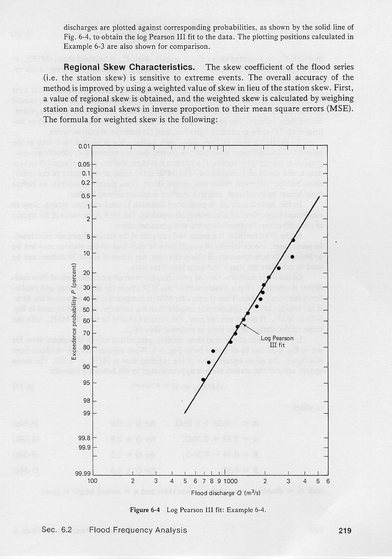
Frequency distibutions are plotted using probability papers.

3.02
One of the scales on a probability paper is a probability scale; the other is either an arithmetic or logarithmic scale.

3.03
Normal and extreme-value probability papers are most often used in frequency analysis.

3.04
A log-probability paper features a normal probability scale and a logarithmic scale.

3.05
A log-probability paper is used to plot Log Pearson distributions.

3.06

3.07
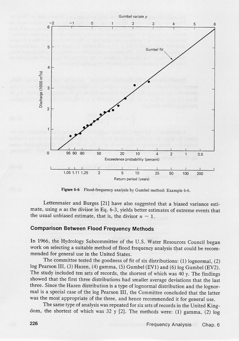
An extreme-value probability paper features an extreme value scale and an arithmetic scale.

3.08
An extreme-value probability paper is used to plot extreme value distributions, among them, notably, the Gumbel distribution.

3.09

3.10
Data fitting a log-normal distribution plot as a straight line on log probability paper.

3.11
Data fitting a Gumbel distribution plot as a straight line on extreme-value probability paper.

3.12
Plotting position formulas enable the plotting of flood series data on probability paper.

3.13
The Weibull plotting position formula is:

3.14

3.15
in which T = return period, P = exceedence probability, m = rank of descending values, and n = number of values in the flood series.

3.16
The Weibull formula is commonly used in hydrologic applications, particularly for computing plotting positions for unspecified distributions.

3.17
A more general plotting position formula is:

3.18

3.19
in which a = parameter.

3.20
The Blom formula, with a = 0.375, is most appropriate for a normal distribution.

3.21
The Gringorten formula, with a = 0.44, applies to the Gumbel distribution.

3.22
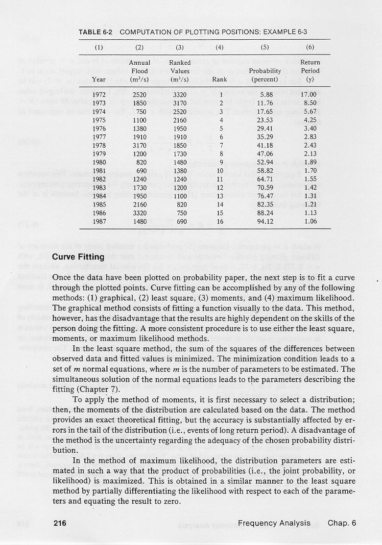
The computation of plotting positions is shown in this table.

3.23

3.24
Column 1 shows the n years in the data series.

3.25
Column 2 shows the flood values, corresponding to each year.

3.26
Column 3 shows the flood values, ranked in descending order.

3.27
Column 4 shows the rank of the values shown in Column 3.

3.28
Column 5 shows the probability, in percent, calculated with the Weibull formula.

3.29
Column 6 shows the return period, in years, calculated with the Weibull formula.

4. CURVE FITTING

4.01
Once the data has been plotted on probability paper, the next step is to fit a curve through the plotted points.

4.02
Curve fitting can be accomplished by any of the following methods: (1) graphical, (2) least square, (3) moments, and (4) maximum likelihood.

4.03
The method of moments is the most widely used curve-fitting method.

4.04
To apply the method of moments, it is necessary to select a distribution; then, the moments of the distribution are calculated based on the data.

4.05
The method provides an exact theoretical fitting, but the accuracy is affected by errors in the tail of the distribution, that is, for events of long return period.

4.06
A disadvantage of the method is the uncertainty regarding the adequacy of the chosen probability distribution.

5. FREQUENCY FACTORS

5.01
The frequency factor is useful in fitting distributions with the method of moments.

5.02
Any random variable can be expressed in terms of the mean and standard deviation as follows:

5.03

5.04
in which K = frequency factor, defined as the difference between the value of the random variable and its mean, divided by the standard deviation.

5.05

5.06
For any probability distribution, a relationship can be determined between frequency factor and return period.

5.07
This relationship can be expressed in analytical terms, in the form of tables, or by a set of K-T curves.

5.08
In practice, K is obtained from the appropriate table, given the return period T, or the associated probability P.

Narrator: Victor M. Ponce

Music: Fernando Oñate

Editor: Flor Pérez

Copyright © 2011

Visualab Productions

All rights reserved