ENGINEERING HYDROLOGY: CHAPTER 063 - FLOOD FREQUENCY METHODS

1. LOG PEARSON III METHOD

1.01
The Log Pearson III method is described in Bulletin 17B: "Guidelines for Determining Flood Flow Frequency," of the U.S. Geological Survey.

1.02
The steps in the application of the Log Pearson III method are the following:

1.03
1. Assemble the annual flood series x_i.

1.04
2. Calculate the logarithms of the annual flood series:

1.05

y_i = log x_i

1.06
3. Calculate the mean, standard deviation, and skew coefficient of the logarithms.

1.07

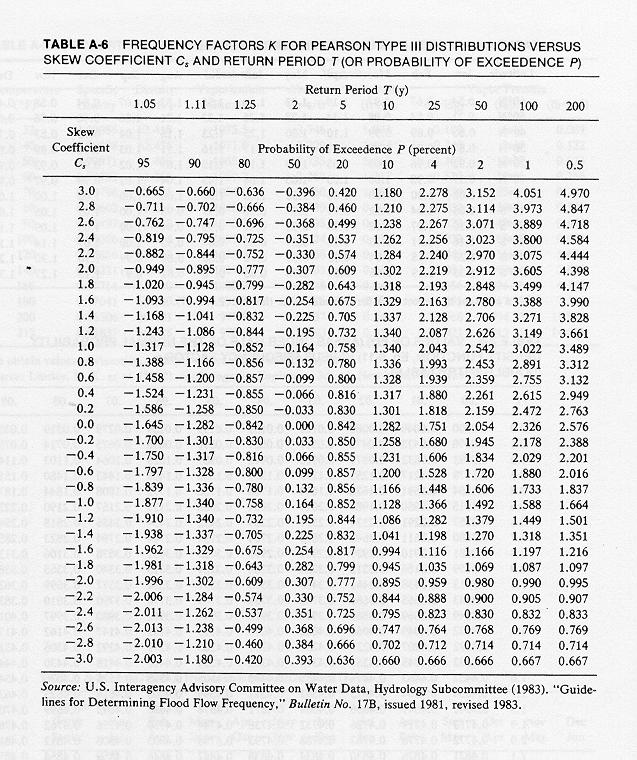
4. Using the double-entry table shown here, calculate the frequency factor for each of several chosen return periods or probability levels, as a function of skew coefficient.

1.08

If necessary, use linear interpolation on the skew coefficient to calculate the applicable frequency factors.

1.09

1.10
5. Calculate the logarithms of the flood discharges using the following frequency formula:

1.11

log Q_j = y + K_j s_y

1.12
in which log Q_j is the logarithm of flood discharge j, y_bar is the mean of the logarithms, K_j is the frequency factor, and s_y is the standard deviation of the logarithms.

1.13
6. Calculate the flood discharges as the antilogarithms of the log Q_j values.

1.14

Q_j = log^-1 (log Q_j)

1.15
7. Plot the flood discharges against probabilities on log probability paper, with discharges on the log scale.

1.16
8. The log Pearson III fit to the data is obtained by linking the points with a smooth curve.

1.17
For skew coefficient equal to zero, the Log Pearson III fit reduces to a straight line.

1.18
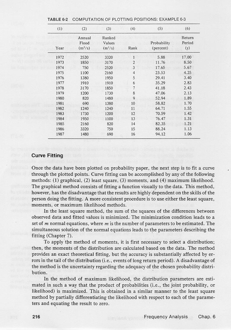
This table shows an example of a flood series and its calculated plotting positions.

1.19

1.20
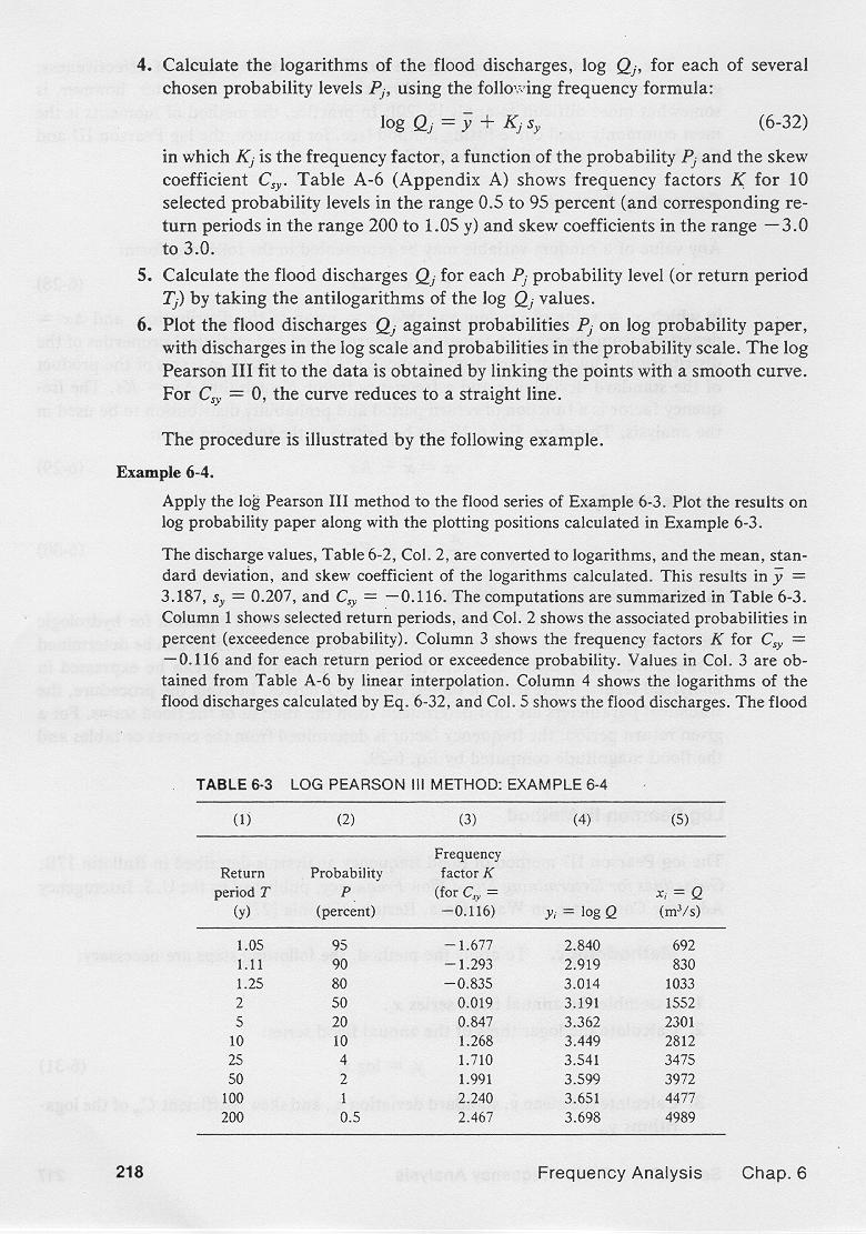
A Log Pearson III fit to this data is shown in this table.

1.21

1.22
Columns 1 and 2 show the selected return periods and associated probabilities, respectively.

1.23
Column 3 shows the frequency factors taken from tha table. For this example, the skew coefficient of the logarithms is C_sy = -0.116.

1.24
Column 4 shows the logarithms of the flood discharges.

1.25
Column 5 shows the calculated flood discharges.

1.26
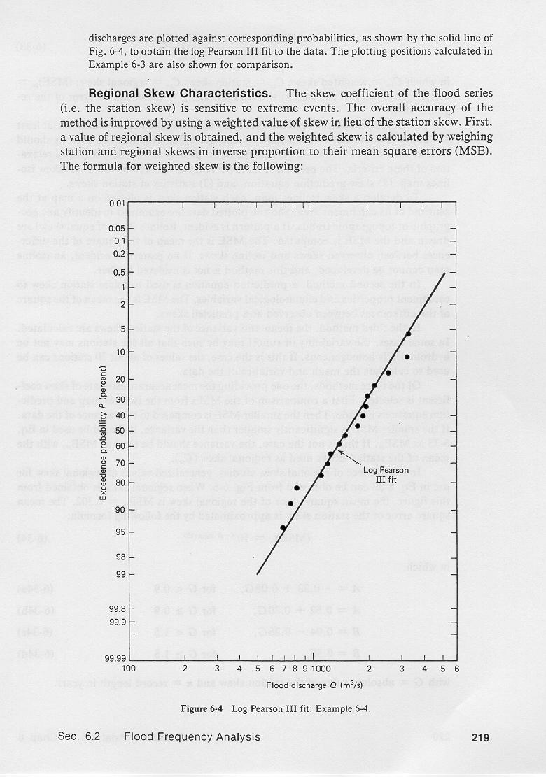
A plot of the Log Pearson Type III fit for the preceding example is shown here.

1.27

2. GUMBEL METHOD

2.01
The Extreme Value Type I distribution, also known as the Gumbel method, or EV1, is in use throughout the world.

2.02
The method is a special case of the three-parameter distribution described in the British Flood Studies Report.

2.03
The cumulative density function of the Gumbel method is the double exponential function:

2.04

F(x) = e^{-e^-y}

2.05
in which F(x) is the probability of nonexceedence.

2.06
In flood frequency analysis, the probability of interest is the probability of exceedence, that is, the complementary probability to F(x), defined as follows:

2.07

G(x) = 1 - F(x)

2.08
The return period is the reciprocal of the probability of exceedence. Therefore:

2.09

1
= 1 - e^{-e^-y}
T

2.10
Solving for y:

2.11

               T
y = - ln ln
             T - 1

2.12
In the Gumbel method, values of flood discharge are obtained from the frequency formula:

2.13

x = x + K s

2.14
The frequency factor K is evaluated with the frequency formula as follows:

2.15

y = y_n + K σ_n

2.16
in which y = Gumbel reduced variate, a function of return period, and y_bar_n and σ_n are the mean and standard deviation of the Gumbel variate.

2.17
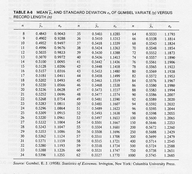
The mean and standard deviation of the Gumbel variate are a function of record length, as shown in this table.

2.18

2.19
For K = 0, the flood discharge is equal to the mean annual flood.

2.20
Also, for K = 0, the Gumbel variate is equal to its mean.

2.21
As the record length n approaches infinity, the mean of the Gumbel variate approaches the value of the Euler constant, that is, 0.5572.

2.22
For y = 0.5572, the return period is T = 2.33 years.

2.23
Therefore, the return period of the mean annual flood is 2.33 years.

2.24
Solving for K:

2.25

      y - y_n
K =
        σ_n

2.26
Replacing this value of K in the flood discharge equation:

2.27

          y - y_n
x = x +
s
            σ_n

2.28
The steps in the application of the Gumbel method are the following:

2.29
1. Assemble the flood series x_i.

2.30
2. Determine the mean and standard deviation of the flood series.

2.31
3. Use this table to determine the mean and standard deviation of the Gumbel variate as a function of record length.

2.32
4. Select several return periods and associated probabilities.

2.33
5. Calculate the Gumbel variates for the selected return periods.

2.34
6. Calculate the flood discharges Q_j = x_j

2.35
7. Plot values of Q against y and/or T or P on Gumbel probability paper, and draw a straight line through the points.

3.36

2.37
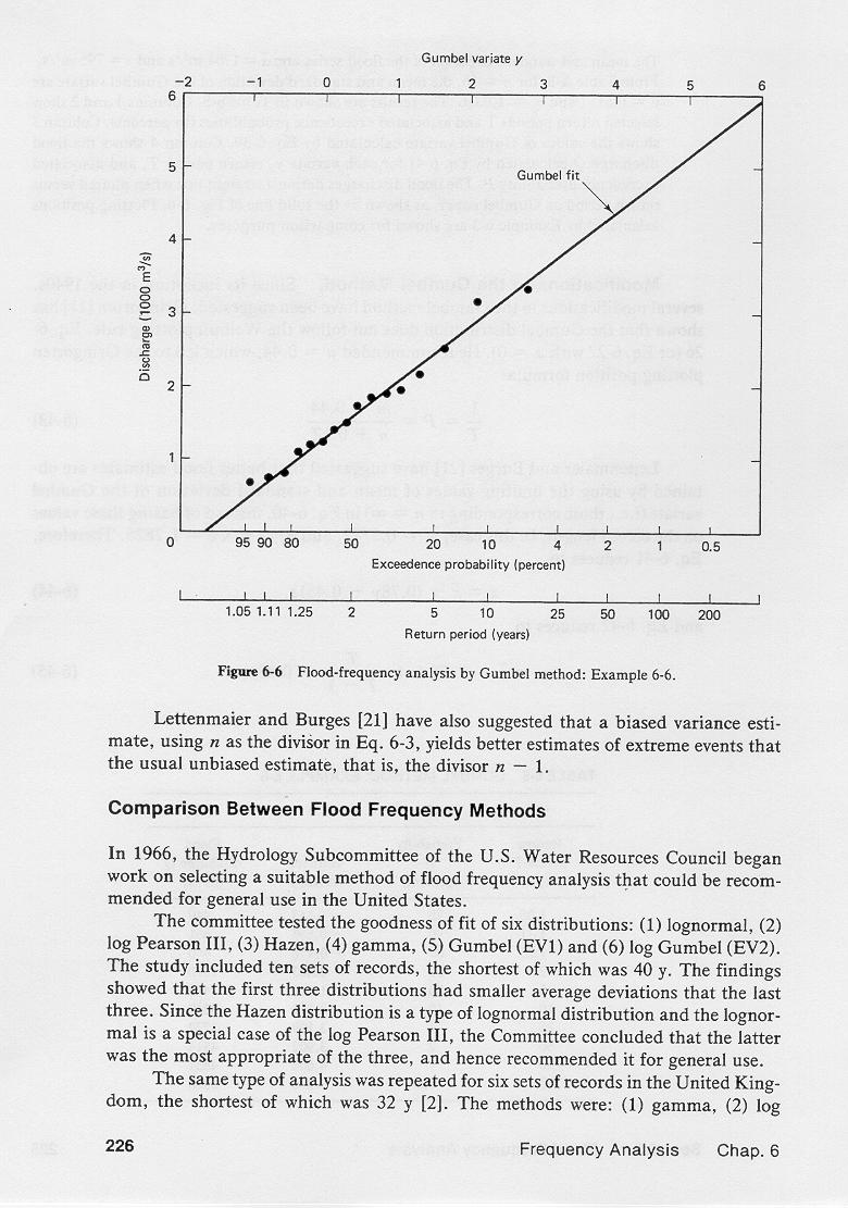
Gumbel probability paper has an arithmetic scale of Gumbel variate in the abscissas, and an arithmetic scale of flood discharge in the ordinates.

2.38
It is customary to superimpose a scale of return period and/or probability on the arithmetic scale of Gumbel variate, as shown here.

2.39
This table shows an example of a flood series and its calculated plotting positions.

2.40

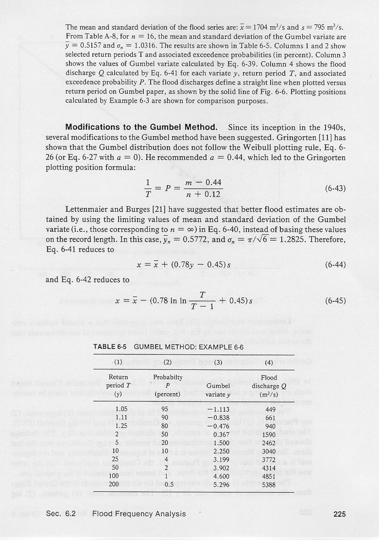
2.41
A Gumbel fit to this data is shown in this table.

3.42

2.43
Columns 1 and 2 show the selected return periods and associated probabilities, respectively.

2.44
Column 3 shows the Gumbel reduced variate.

2.45
Column 4 shows the flood discharges.

2.46
The Gringorten plotting position formula is preferred for use with the Gumbel method.

2.47
The Gringorten formula is:

2.48

1         m - 0.44
= P =
T         n + 0.12

3. COMPARISON OF METHODS

3.01
In 1968, the Hydrology Subcommitee of the U.S. Water Resources Council tested the goodness of fit of six frequency distributions.

3.02
These were: (1) Lognormal, (2) Log Pearson III, (3) Hazen, (4) Gamma, (5) Gumbel, and (6) Log Gumbel.

3.03
The study showed that the first three distributions had smaller average deviations that the other three.

3.04
Since the Hazen distribution is a type of lognormal, and the lognormal is a special case of the Log Pearson III, the Committee concluded that the Log Pearson III distribution was the most appropriate, and recommended it for general use.

3.05
The British Flood Studies Report of 1975 concluded that the three-parameter distributions, that is Log Pearson III and Generalized Extreme Value, or GEV, provided a better fit than the two-parameter distributions, such as lognormal and Gumbel.

3.06
However, the same report noted that the use of two-parameter distributions in connection with short record lengths often leads to results that are more sensible than those obtained by fitting three-parameter distributions.

4. COMPLEMENTS TO FLOOD FREQUENCY ESTIMATES

4.01
The accuracy of flood estimates based on frequency analysis deteriorates for values of probability much greater than the record length.

4.02
This is due to sampling errors and to the fact that the underlying distribution is not known with certainty.

4.03
Alternative procedures that complement the information provided by flood frequency analysis are recommended.

4.04
These procedures include flood estimates from precipitation and comparison with catchments of similar hydrologic characteristics.

4.05
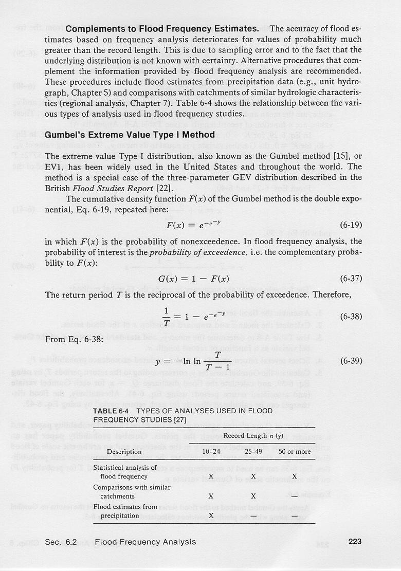
This table shows the relation between the various types of analysis used in flood frequency studies.

4.06
For short record lengths, the three methods complement each other, while for long record lengths, the statistical method is applicable.

4.07

Narrator: Victor M. Ponce
Music: Fernando Oñate
Editor: Flor Pérez

Copyright © 2011
Visualab Productions
All rights reserved