ENGINEERING HYDROLOGY: CHAPTER 072 - REGRESSION ANALYSIS

1. BIVARIATE NORMAL DISTRIBUTION

1.01
The bivariate normal distribution is the foundation of regression theory.

1.02
The bivariate normal distribution is:

1.03

f(x, y) = K e^M

1.04
in which x and y are the random variables.

1.05
The parameters K and M are a function of the means μ_x and μ_y, the standard deviations σ_x and σ_y, and the correlation coefficient ρ.

1.06
The conditional distribution is obtained by dividing the bivariate normal by the univariate normal, to yield:

1.07

f(x|y) = K' e^M'

1.08
As in the case of the bivariate normal, for the conditional normal, the parameters K' and M' are a function of the means, the standard deviations, and the correlation coefficient.

1.09
The conditional normal distribution has the following mean:

1.10

              σ_y
μ_y|x = μ_y + ρ
(x - μ_x)
              σ_x

1.11
This equation expresses the linear dependence between x and y.

1.12
The slope of the regression line is:

1.13

       σ_y
β = ρ
       σ_x

1.14
The conditional normal distribution has the following variance:

1.15

σ_e² = σ_y² (1 - ρ²)

1.16
The correlation coefficient ρ is the fraction of the original variance explained or removed by the regression.

1.17
For ρ = 1, all the variance is removed.

1.18
For ρ = 0, all the variance remains.

2. ONE-PREDICTOR-VARIABLE REGRESSION

2.01
Assume two or more random variables that are related.

2.02
The variable for which values are given is called the predictor variable.

2.03
The variable for which values must be estimated is called the criterion variable.

2.04
The equation relating criterion and predictor variables is the prediction equation.

2.05
The objective of regression analysis is to evaluate the parameters of the prediction equation.

2.06
Correlation provides a measure of the goodness of fit of the regression.

2.07
Therefore, while regression provides the parameters of the prediction equation, correlation describes its quality.

2.08
This distinction is necessary because the predictor and criterion variables cannot be switched, unless the correlation coefficient is equal to 1.

2.09
In hydrologic modeling, regression analysis is useful in model calibration; correlation is useful in model formulation and verification.

2.10
The principle of least squares is used in regression analysis as a means of obtaining the best estimate of the parameters of the prediction equation.

2.11
The principle is based on the minimization of the sum of the squares of the differences between observed and predicted values.

2.12
The procedure can be used to regress one criterion variable on one or more predictor variables.

2.13
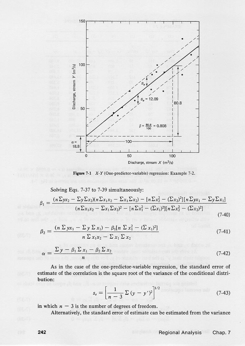
In one-predictor-variable regression, the line to be fitted has the following form:

2.14

y' = α + β x

2.15
The sum of the squares of the differences between y and y' are minimized.

2.16

∑ (y - y')² = ∑ [y - (α + β x)]²

2.17
This leads to the parameters of the regression:

2.18

      ∑xy - (∑x ∑y)/n
β =
       ∑x² - (∑x)²/n

2.19

      ∑y - β ∑x
α =
          n

2.20
Since the slope of the regression line is

2.21

       σ_y
β = ρ
       σ_x

2.22
the estimate from sample data is:

2.23

       s_y
β = r
       s_x

2.24
Therefore, the correlation coefficient is:

2.25

       s_x
r = β
       s_y

2.26
The standard error of estimate is the variance of the conditional distribution.

2.27
For calculations based on sample data, the standard error of estimate is:

2.28

          n - 1
s_e = s_y [
(1 - r²)]^1/2
          n - 2

2.29

2.30
The regression equations can be used to fit power functions of the type:

2.31

y = a x^b

2.32
This equation is linearized by taking the logarithms:

2.33

log y = log a + b log x

2.34
With u = log x, and v = log y, this equation is:

2.35

v = log a + b u

2.36
Replacing x and y for u and v in the equations for the regression parameters, leads to:

2.37

y = 10^α x^β

3. MULTIPLE REGRESSION

3.01
Multiple regression is the extension of the least squares technique to more than one predictor variable.

3.02
For the case of two predictor variables, the line to be fitted is:

3.03

y' = α + β₁ x₁ + β₂ x₂

3.04
The sum of the squares of the differences between the criterion variable y and its estimate y' is:

3.05

∑ (y - y')² = ∑ [y - (α + β₁ x₁ + β₂ x₂)]²

3.06
The minimization of the sum of the squares leads to equations for α, β₁, and β₂, as a function of the predictor variables x₁ and x₂ and criterion variable y.

3.07

      (n∑yx₂ - ∑y∑x₂)(n∑x₁x₂ - ∑x₁∑x₂) - [n∑x₂² - (∑x₂)²][n∑yx₁ - ∑y∑x₁]
β₁ =
             (n∑x₁x₂ - ∑x₁∑x₂)² - [n∑x₁² - (∑x₁)²][n∑x₂² - (∑x₂)²]

3.08

      (n∑yx₁ - ∑y∑x₁) - β₁[n∑x₁² - (∑x₁)²]
β₂ =
                n∑x₁x₂ - ∑x₁∑x₂

3.09

      ∑y - β₁∑x₁ - β₂∑x₂
α =
               n

3.10
The multiple regression equations can be used to fit power functions of the type:

3.11

y = a x₁^b₁ x₂^b₂

3.12
This equation is linearized by taking the logarithms:

3.13

log y = log a + b₁ log x₁ + b₂ log x₂

3.14
With u = log x₁, v = log x₂, and w = log y, this equation is:

3.15

w = log a + b u + c v

3.16
Replacing x₁, x₂, and y for u, v and w in the equations for the regression parameters, leads to:

3.17

y = 10^α x₁^β₁ x₂^β₂

Narrator: Victor M. Ponce
Music: Fernando Oñate
Editor: Flor Pérez

Copyright © 2011
Visualab Productions
All rights reserved