1. PEAK FLOW FORMULAS

1.01
Regional analysis encompasses the study of hydrologic phenomena with the aim of developing mathematical relations to be used in a regional context.

1.02
The earliest approach to regionalization of hydrologic properties was to assume that flood peak discharge is related to catchment area, and to perform a regression to determine the parameters.

1.03
The typical equation is of the following form:

1.04

1.05
in which Q_p = flood peak discharge;
A = catchment area, and
c and m are regression constants.

1.06
In nature, as catchment area increases, the spatially averaged rainfall intensity decreases and, consequently, flood peak discharge does not increase as fast as catchment area.

1.07
Therefore, the exponent m is always less than unity, usually in the range 0.4 to 0.9.

1.08
Other formulas relating peak flow to catchment area are the following:

1.09

1.10

1.11

1.12
in which a, b, c, d, m, and n are parameters determined from statistical analysis of measured data and are applicable on a regional basis, that is, for neighboring catchments of similar physiographic, vegetative, and land-use patterns.

1.13
The Creager curves are an example of the first equation.

1.14
In principle, none of these equations accounts explicitly for flood frequency, being limited to providing a maximum flow.

1.15
However, as in the Creager curves, the effect of flood frequency can be accounted for by varying the parameters.

2. USGS STATE EQUATIONS

2.01
The U.S. Geological Survey uses multiple regression techniques to determine flood frequency at ungaged sites.

2.02
These techniques are based on statistical regression to relate flood magnitude and frequency to watershed and climatic characteristics.

2.03
The predictive equations have the following general form:

2.04

2.05
in which Q is a flood peak associated with a given frequency, b(i = 0,1,2, ...,k) are regression constants determined by least squares, X_i are watershed and climatic characteristics, and k is generally less than 7.

2.06
An example of the USGS State equations for the State of California's South Coast Region are:

2.07

2.08
in which A = drainage area, in square miles, and P = mean annual precipitation, in inches.

2.09
Similar formulas are available for other California regions, and other states in the United States.

2.10
The accuracy of the USGS state equations is variable across the United States.

2.11
The quality of the prediction decreases in the Western United States, due to greater variability in annual flood series and the sparsity of the sampling network.

3. INTENSITY-DURATION-FREQUENCY CURVES

3.01
Curves showing the relationship between intensity, duration, and frequency of rainfall are required for peak flow computations in small catchments.

3.02
These curves can be developed using regional or local rainfall intensity-duration data.

3.03
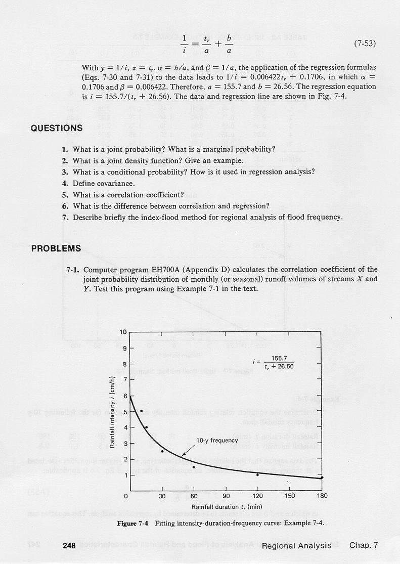
The following hyperbolic equation is applicable:

3.04

3.05
in which i = rainfall intensity, t_r = rainfall duration, and a and b are constants to be determined by regression analysis.

3.06
The applicable linear equation is:

3.07

3.08
The hyperbolic intensity-duration equation is linearized in the following way:

3.09

3.10
Comparing these two equations leads to:

3.11

3.12
The application of the regression equations enables the calculation of the intensity-duration parameters a and b.

3.13
The repetition of the procedure for other frequencies leads to the intensity-duration frequency curve, or IDF curve.

3.14

Narrator: Victor M. Ponce

Music: Fernando Oñate

Editor: Flor Pérez

Copyright © 2011

Visualab Productions

All rights reserved