|
ENGINEERING HYDROLOGY: CHAPTER 103 - CASCADE OF LINEAR RESERVOIRS
1. RATIONALE
1.01
A linear reservoir has a diffusive effect on the inflow hydrograph.
1.02
If an inflow hydrograph is routed through a linear reservoir,
the outflow hydrograph has a reduced peak and an increased time base.
1.03
The increase in time base causes a difference in the relative timing of
inflow and outflow hydrographs.
1.04
This timing is referred to as the lag.
1.05
The amount of diffusion and associated lag is a function of the ratio
Δt/K, a larger diffusion effect corresponding to smaller values
of Δt/K.
1.06
The cascade of linear reservoirs is a widely used method of hydrologic
catchment routing.
1.07
As its name implies, the method is based on the connection of several
linear reservoirs in series.
1.08
For N such reservoirs, the outflow from the first would be taken as inflow
to the second, the outflow from the second as inflow to the third,
and so on, until the outflow from the (N-1) reservoir is taken as the inflow
to the Nth reservoir.
1.09
The outflow from the last reservoir is the outflow from the cascade.
1.10
Admittedly, the cascade of reservoirs to simulate catchment response
is an abstract concept.
1.11
Nevertheless, it has proven to be quite useful in practice.
1.12
Each reservoir in the series provides a certain amount of diffusion
and associated lag.
1.13
For a given set of parameters, Δt/K and N, the outflow from the
last reservoir is a function of the inflow to the first reservoir.
1.14
In this way, a one-parameter linear reservoir method, with Δt/K
as a parameter, is extended to a two-parameter catchment routing method,
adding N as the second parameter.
1.15
Moreover, the routing formula and routing coefficients remain
the same as those of the linear reservoir method.
1.16
The addition of a second parameter, N,
provides considerable flexibility for simulating a wide range of diffusion
and associated lag effects.
1.17
However, the conceptual basis of the method restricts is general use,
since there is no clear
relation between either of the parameters and the physical
problem.
1.18
Notwithstanding this apparent limitation, the cascade of linear reservoirs
has been widely used in catchment routing, particularly for applications
to large gaged river basins.
1.19
Rainfall-runoff data can be used to calibrate the method, that is,
to determine a set of parameters Δt/K and N
that produces the best fit to the measured data.
1.20
The analytical version of the cascade of linear reservoirs is referred to
as the Nash model.
1.21
The numerical version is featured in several hydrologic simulation
models developed in the United States and other countries.
1.22
Notable among them is the Streamflow Synthesis and Reservoir Regulation
model, or SSARR model, of the U.S. Army Corps of Engineers.
2. METHODOLOGY
2.01
To derive the routing equation for the cascade of linear reservoirs,
the routing equation for a single linear reservoir is expressed as follows:
2.02
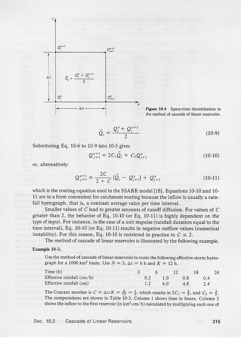
n+1 n+1 n n
| Qj+1 = C0 Qj
+ C1 Qj + C2 Qj+1 |
|
2.03
in which Q represents discharge, whether inflow or outflow, and j and n are
space and time indexes, respectively, as shown here.
2.04
The routing coefficients are a function of the dimensionless ratio
Δt/K.
2.05
This ratio is interpreted as a Courant number, defined as follows:
2.06
2.07
In terms of Courant number, the routing coefficients are expressed as follows:
2.08
2.09
2.10
2.11
For application to catchment routing,
for which the first inflow is a hyetograph,
the average inflow is:
2.12
2.13
In terms of average inflow and initial outflow, the routing equation
converts to:
2.14
2.15
This equation is the routing equation of the cascade of linear reservoirs,
particularly applicable to catchment routing.
2.16
Through an algebraic manipulation, it can be recast as follows:
2.17
n+1 2 C _ n n
| Qj+1 = |
|
[Qj - Qj+1] + Qj+1
|
2 + C
|
2.18
This equation is the routing equation of the SSARR model.
2.19
In practice, the Courant number is restricted in the range 0-2.
2.20
Smaller values of C lead to greater amounts of runoff diffusion;
conversely, larger values of C lead to smaller amounts to runoff diffusion.
2.21
Values of C greater than 2 are not recommended, because it may lead
to unrealistic negative outflows.
3. EXAMPLE
3.01
In this example, we use the method of cascade of linear reservoirs
to route an effective storm hyetograph through a 1000 km2.
3.02
We use N = 3, Δt = 6 hr, and K = 12 hr.
3.03
The effective rainfall hyetograph is the following:
3.04
Effective rainfall hyetograph
| Time (hr)
| 6
| 12
| 18
| 24
|
| Effective rainfall (cm/hr)
| 0.2
| 1.0
| 0.8
| 0.4
|
| Effective rainfall (cm)
| 1.2
| 6.0
| 4.8
| 2.4
|
|
3.05
The Courant number is:
3.06
3.07
which results in:
3.08
3.09
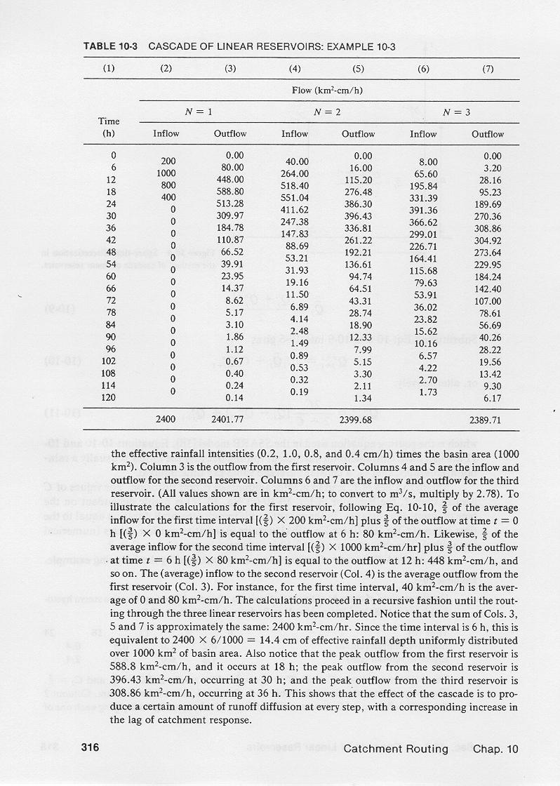
The computations are shown in this table.
3.10
Column 1 shows the time in hours.
3.11
Column 2 shows the inflow to the first reservoir, in km2-cm/hr,
calculated by multiplying each one of the effective rainfall intensities times the
basin area, which is 1000 km2.
3.12
Column 3 is the outflow from the first reservoir, calculated with the routing equation
shown here.
3.13
Column 4 is the inflow to the second reservoir, calculated
as the average of the outflows from the first reservoir.
3.14
Column 5 is the outflow from the second reservoir.
3.15
Column 6 is the inflow to the third reservoir.
3.16
Column 7 is the outflow from the third reservoir.
3.17
Column 7 is the outflow from the cascade, in km2-ch/hr.
3.18
To convert this outflow to m3/s, multiply the values of Column 7 by 2.78.
3.19
To illustrate the calculations for the first reservoir,
2/5 of the average inflow for the first time interval, that is, 200,
plus to 3/5 of the outflow at time t = 0, that is 0, is equal to the outflow at time t = 1, that is, 80.
3.20
| [(2/5) × 200] + [(3/5) × 0] = 80 |
|
3.21
The average inflow to the second reservoir is the average outflow from the first reservoir.
For the first time interval, the average of 0 and 80
is equal to 40.
3.22
3.23
Note that the sum of Columns 3, 5, and 7 is approximately the same, that is,
2400 km2-cm/hr.
3.24
This amounts to 14.4 cm of effective rainfall depth uniformly
distributed over the entire basin.
3.25
Note that the peak outflow from the first reservoir is 588.8, and it occurs
at 18 hr.
3.26
The peak outflow from the second reservoir is 396.43, and it occurs at 30 hr.
3.27
The peak outflow from the third reseevoir is 308.86, and it occurs at 36 hr.
3.28
These results show that the effect of the cascade is to provide a certain amount of
diffusion at every step, with a corresponding increase in the lag of catchment response.
4. ASSESSMENT
4.01
The cascade of linear reservoirs provides a convenient procedure for simulating
a wide range of catchment routing problems.
4.02
Furthermore, the method can be applied separately to each runoff
component; (1) surface runoff, (2) subsurface runoff, and (3) baseflow.
4.03
In this case, the catchment response is taken as the sum of the responses of the
individual components.
4.04
For instance, assume that a certain basin has 10 cm of runoff, of which 7 cm are surface
runoff, 2 cm are subsurface runoff, and 1 cm is baseflow.
4.05
Since surface runoff is less diffused, it can be simulated with a high Courant number, say
C = 1, and a small number of reservoirs, say, N = 3.
4.06
Being more diffused that surface runoff, subsurface runoff can be simulated with C = 0.4 and N = 5.
Baseflow being the most diffused, can be simulated with C = 0.1 and N = 7.
4.07
In practice, the parameters C and N are determined by extensive calibration.
4.08
In this sense, the cascade of linear reservoirs remains essentially a conceptual model.
4.09

4.10

Narrator: Victor M. Ponce
Music: Fernando Oñate
Editor: Flor Pérez
Copyright © 2011
Visualab Productions
All rights reserved
| 
